Hashtable Online Tutorials
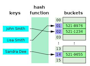
In computing, a hash table, also known as a hash map or a hash set, is a data structure that implements an associative array, also called a dictionary, which is an abstract data type that maps keys to values. A hash table uses a hash function to compute an index, also called a hash code, into an array of buckets or slots, from which the desired value can be found. During lookup, the key is hashed and the resulting hash indicates where the corresponding value is stored.
| Hash table | ||||||||||||||||||||||||
|---|---|---|---|---|---|---|---|---|---|---|---|---|---|---|---|---|---|---|---|---|---|---|---|---|
| Type | Unordered associative array | |||||||||||||||||||||||
| Invented | 1953 | |||||||||||||||||||||||
| ||||||||||||||||||||||||
Ideally, the hash function will assign each key to a unique bucket, but most hash table designs employ an imperfect hash function, which might cause hash collisions where the hash function generates the same index for more than one key. Such collisions are typically accommodated in some way.
In a well-dimensioned hash table, the average time complexity for each lookup is independent of the number of elements stored in the table. Many hash table designs also allow arbitrary insertions and deletions of key–value pairs, at amortized constant average cost per operation.
Hashing is an example of a space-time tradeoff. If memory is infinite, the entire key can be used directly as an index to locate its value with a single memory access. On the other hand, if infinite time is available, values can be stored without regard for their keys, and a binary search or linear search can be used to retrieve the element.: 458
In many situations, hash tables turn out to be on average more efficient than search trees or any other table lookup structure. For this reason, they are widely used in many kinds of computer software, particularly for associative arrays, database indexing, caches, and sets.
History edit
The idea of hashing arose independently in different places. In January 1953, Hans Peter Luhn wrote an internal IBM memorandum that used hashing with chaining. The first example of open addressing was proposed by A. D. Linh, building on Luhn's memorandum.: 547 Around the same time, Gene Amdahl, Elaine M. McGraw, Nathaniel Rochester, and Arthur Samuel of IBM Research implemented hashing for the IBM 701 assembler.: 124 Open addressing with linear probing is credited to Amdahl, although Andrey Ershov independently had the same idea.: 124–125 The term "open addressing" was coined by W. Wesley Peterson on his article which discusses the problem of search in large files.: 15
The first published work on hashing with chaining is credited to Arnold Dumey, who discussed the idea of using remainder modulo a prime as a hash function.: 15 The word "hashing" was first published in an article by Robert Morris.: 126 A theoretical analysis of linear probing was submitted originally by Konheim and Weiss.: 15
Overview edit
An associative array stores a set of (key, value) pairs and allows insertion, deletion, and lookup (search), with the constraint of unique keys. In the hash table implementation of associative arrays, an array of length is partially filled with elements, where . A value gets stored at an index location , where is a hash function, and .: 2 Under reasonable assumptions, hash tables have better time complexity bounds on search, delete, and insert operations in comparison to self-balancing binary search trees.: 1


Hash tables are also commonly used to implement sets, by omitting the stored value for each key and merely tracking whether the key is present.: 1
Load factor edit
A load factor is a critical statistic of a hash table, and is defined as follows:


- is the number of entries occupied in the hash table.
- is the number of buckets.
The performance of the hash table deteriorates in relation to the load factor .: 2
To maintain good performance, the software makes sure the load factor never exceeds some constant .

Therefore a hash table is resized or rehashed whenever the load factor reaches .
A table is also resized if the load factor drops below .

Load factor for separate chaining edit
With separate chaining hash tables, each slot of the bucket array stores a pointer to a list or array of data.
Separate chaining hash tables suffer gradually declining performance as the load factor grows, and no fixed point beyond which resizing is absolutely needed.
With separate chaining, the value of that gives best performance is typically between 1 and 3.
Load factor for open addressing edit
With open addressing, each slot of the bucket array holds exactly one item. Therefore an open-addressed hash table cannot have a load factor greater than 1.
The performance of open addressing becomes very bad when the load factor approaches 1.
Therefore a hash table that uses open addressing must be resized or rehashed if the load factor approaches 1.
With open addressing, acceptable figures of max load factor should range around 0.6 to 0.75.: 110
Hash function edit
A hash function maps the universe of keys to indices or slots within the table, that is, for . The conventional implementations of hash functions are based on the integer universe assumption that all elements of the table stem from the universe , where the bit length of is confined within the word size of a computer architecture.: 2


A hash function is said to be perfect for a given set if it is injective on , that is, if each element maps to a different value in . A perfect hash function can be created if all the keys are known ahead of time.


Integer universe assumption edit
The schemes of hashing used in integer universe assumption include hashing by division, hashing by multiplication, universal hashing, dynamic perfect hashing, and static perfect hashing.: 2 However, hashing by division is the commonly used scheme.: 264 : 110
Hashing by division edit
The scheme in hashing by division is as follows:: 2


Hashing by multiplication edit
The scheme in hashing by multiplication is as follows:: 2–3

Choosing a hash function edit
Uniform distribution of the hash values is a fundamental requirement of a hash function. A non-uniform distribution increases the number of collisions and the cost of resolving them. Uniformity is sometimes difficult to ensure by design, but may be evaluated empirically using statistical tests, e.g., a Pearson's chi-squared test for discrete uniform distributions.
The distribution needs to be uniform only for table sizes that occur in the application. In particular, if one uses dynamic resizing with exact doubling and halving of the table size, then the hash function needs to be uniform only when the size is a power of two. Here the index can be computed as some range of bits of the hash function. On the other hand, some hashing algorithms prefer to have the size be a prime number.
For open addressing schemes, the hash function should also avoid clustering, the mapping of two or more keys to consecutive slots. Such clustering may cause the lookup cost to skyrocket, even if the load factor is low and collisions are infrequent. The popular multiplicative hash is claimed to have particularly poor clustering behavior.
K-independent hashing offers a way to prove a certain hash function does not have bad keysets for a given type of hashtable. A number of K-independence results are known for collision resolution schemes such as linear probing and cuckoo hashing. Since K-independence can prove a hash function works, one can then focus on finding the fastest possible such hash function.
Collision resolution edit
A search algorithm that uses hashing consists of two parts. The first part is computing a hash function which transforms the search key into an array index. The ideal case is such that no two search keys hashes to the same array index. However, this is not always the case and is impossible to guarantee for unseen given data.: 515 Hence the second part of the algorithm is collision resolution. The two common methods for collision resolution are separate chaining and open addressing.: 458
Separate chaining edit
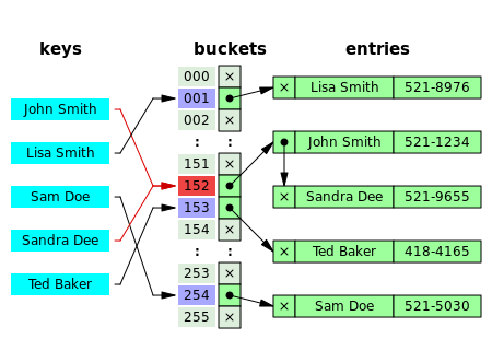

In separate chaining, the process involves building a linked list with key–value pair for each search array index. The collided items are chained together through a single linked list, which can be traversed to access the item with a unique search key.: 464 Collision resolution through chaining with linked list is a common method of implementation of hash tables. Let and be the hash table and the node respectively, the operation involves as follows:: 258

Chained-Hash-Insert(T, k)
  insert x at the head of linked list T

Chained-Hash-Search(T, k)
  search for an element with key k in linked list T

Chained-Hash-Delete(T, k)
  delete x from the linked list T
If the element is comparable either numerically or lexically, and inserted into the list by maintaining the total order, it results in faster termination of the unsuccessful searches.: 520–521
Other data structures for separate chaining edit
If the keys are ordered, it could be efficient to use "self-organizing" concepts such as using a self-balancing binary search tree, through which the theoretical worst case could be brought down to , although it introduces additional complexities.: 521

In dynamic perfect hashing, two-level hash tables are used to reduce the look-up complexity to be a guaranteed in the worst case. In this technique, the buckets of entries are organized as perfect hash tables with slots providing constant worst-case lookup time, and low amortized time for insertion. A study shows array-based separate chaining to be 97% more performant when compared to the standard linked list method under heavy load.: 99


Techniques such as using fusion tree for each buckets also result in constant time for all operations with high probability.
Caching and locality of reference edit
The linked list of separate chaining implementation may not be cache-conscious due to spatial locality—locality of reference—when the nodes of the linked list are scattered across memory, thus the list traversal during insert and search may entail CPU cache inefficiencies.: 91
In cache-conscious variants of collision resolution through separate chaining, a dynamic array found to be more cache-friendly is used in the place where a linked list or self-balancing binary search trees is usually deployed, since the contiguous allocation pattern of the array could be exploited by hardware-cache prefetchers—such as translation lookaside buffer—resulting in reduced access time and memory consumption.
Open addressing edit
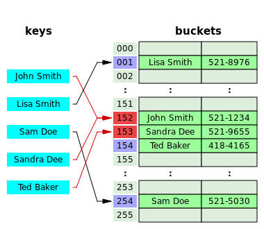

Open addressing is another collision resolution technique in which every entry record is stored in the bucket array itself, and the hash resolution is performed through probing. When a new entry has to be inserted, the buckets are examined, starting with the hashed-to slot and proceeding in some probe sequence, until an unoccupied slot is found. When searching for an entry, the buckets are scanned in the same sequence, until either the target record is found, or an unused array slot is found, which indicates an unsuccessful search.
Well-known probe sequences include:
- Linear probing, in which the interval between probes is fixed (usually 1).
- Quadratic probing, in which the interval between probes is increased by adding the successive outputs of a quadratic polynomial to the value given by the original hash computation.: 272
- Double hashing, in which the interval between probes is computed by a secondary hash function.: 272–273
The performance of open addressing may be slower compared to separate chaining since the probe sequence increases when the load factor approaches 1.[22]: 93 The probing results in an infinite loop if the load factor reaches 1, in the case of a completely filled table.[6]: 471 The average cost of linear probing depends on the hash function's ability to distribute the elements uniformly throughout the table to avoid clustering, since formation of clusters would result in increased search time.[6]: 472
Caching and locality of reference edit
Since the slots are located in successive locations, linear probing could lead to better utilization of CPU cache due to locality of references resulting in reduced memory latency.[28]
Other collision resolution techniques based on open addressing edit
Coalesced hashing edit
Coalesced hashing is a hybrid of both separate chaining and open addressing in which the buckets or nodes link within the table.[30]: 6–8 The algorithm is ideally suited for fixed memory allocation.[30]: 4 The collision in coalesced hashing is resolved by identifying the largest-indexed empty slot on the hash table, then the colliding value is inserted into that slot. The bucket is also linked to the inserted node's slot which contains its colliding hash address.[30]: 8
Cuckoo hashing edit
Cuckoo hashing is a form of open addressing collision resolution technique which guarantees worst-case lookup complexity and constant amortized time for insertions. The collision is resolved through maintaining two hash tables, each having its own hashing function, and collided slot gets replaced with the given item, and the preoccupied element of the slot gets displaced into the other hash table. The process continues until every key has its own spot in the empty buckets of the tables; if the procedure enters into infinite loop—which is identified through maintaining a threshold loop counter—both hash tables get rehashed with newer hash functions and the procedure continues.[31]: 124–125
Hopscotch hashing edit
Hopscotch hashing is an open addressing based algorithm which combines the elements of cuckoo hashing, linear probing and chaining through the notion of a neighbourhood of buckets—the subsequent buckets around any given occupied bucket, also called a "virtual" bucket.[32]: 351–352 The algorithm is designed to deliver better performance when the load factor of the hash table grows beyond 90%; it also provides high throughput in concurrent settings, thus well suited for implementing resizable concurrent hash table.[32]: 350 The neighbourhood characteristic of hopscotch hashing guarantees a property that, the cost of finding the desired item from any given buckets within the neighbourhood is very close to the cost of finding it in the bucket itself; the algorithm attempts to be an item into its neighbourhood—with a possible cost involved in displacing other items.[32]: 352
Each bucket within the hash table includes an additional "hop-information"—an H-bit bit array for indicating the relative distance of the item which was originally hashed into the current virtual bucket within H-1 entries.[32]: 352 Let and be the key to be inserted and bucket to which the key is hashed into respectively; several cases are involved in the insertion procedure such that the neighbourhood property of the algorithm is vowed:[32]: 352–353 if is empty, the element is inserted, and the leftmost bit of bitmap is set to 1; if not empty, linear probing is used for finding an empty slot in the table, the bitmap of the bucket gets updated followed by the insertion; if the empty slot is not within the range of the neighbourhood, i.e. H-1, subsequent swap and hop-info bit array manipulation of each bucket is performed in accordance with its neighbourhood invariant properties.[32]: 353

Robin Hood hashing edit
Robin Hood hashing is an open addressing based collision resolution algorithm; the collisions are resolved through favouring the displacement of the element that is farthest—or longest probe sequence length (PSL)—from its "home location" i.e. the bucket to which the item was hashed into.[33]: 12 Although Robin Hood hashing does not change the theoretical search cost, it significantly affects the variance of the distribution of the items on the buckets,[34]: 2 i.e. dealing with cluster formation in the hash table.[35] Each node within the hash table that uses Robin Hood hashing should be augmented to store an extra PSL value.[36] Let be the key to be inserted, be the (incremental) PSL length of , be the hash table and be the index, the insertion procedure is as follows:[33]: 12–13 [37]: 5


- If : the iteration goes into the next bucket without attempting an external probe.
- If : insert the item into the bucket ; swap with —let it be ; continue the probe from the st bucket to insert ; repeat the procedure until every element is inserted.
![{\displaystyle x.psl\ \leq \ T[j].psl}](https://wikimedia.org/api/rest_v1/media/math/render/svg/0813eb6a21c2c8a817aa86085d3cf9417f01e8fb)
![{\displaystyle x.psl\ >\ T[j].psl}](https://wikimedia.org/api/rest_v1/media/math/render/svg/d06f4753fda641edd5afb066239100a667124f39)
![{\displaystyle T[j]}](https://wikimedia.org/api/rest_v1/media/math/render/svg/cb1f9ca1ed801caf88d5004aa3685644667099b6)


Dynamic resizing edit
Repeated insertions cause the number of entries in a hash table to grow, which consequently increases the load factor; to maintain the amortized performance of the lookup and insertion operations, a hash table is dynamically resized and the items of the tables are rehashed into the buckets of the new hash table,[9] since the items cannot be copied over as varying table sizes results in different hash value due to modulo operation.[38] If a hash table becomes "too empty" after deleting some elements, resizing may be performed to avoid excessive memory usage.[39]
Resizing by moving all entries edit
Generally, a new hash table with a size double that of the original hash table gets allocated privately and every item in the original hash table gets moved to the newly allocated one by computing the hash values of the items followed by the insertion operation. Rehashing is simple, but computationally expensive.[40]: 478–479
Alternatives to all-at-once rehashing edit
Some hash table implementations, notably in real-time systems, cannot pay the price of enlarging the hash table all at once, because it may interrupt time-critical operations. If one cannot avoid dynamic resizing, a solution is to perform the resizing gradually to avoid storage blip—typically at 50% of new table's size—during rehashing and to avoid memory fragmentation that triggers heap compaction due to deallocation of large memory blocks caused by the old hash table.[41]: 2–3 In such case, the rehashing operation is done incrementally through extending prior memory block allocated for the old hash table such that the buckets of the hash table remain unaltered. A common approach for amortized rehashing involves maintaining two hash functions and . The process of rehashing a bucket's items in accordance with the new hash function is termed as cleaning, which is implemented through command pattern by encapsulating the operations such as , and through a wrapper such that each element in the bucket gets rehashed and its procedure involve as follows:[41]: 3


- Clean bucket.
- Clean bucket.
- The command gets executed.
![{\displaystyle \mathrm {Table} [h_{\text{old}}(\mathrm {key} )]}](https://wikimedia.org/api/rest_v1/media/math/render/svg/afcb195bb40a51be98c16b6d9b930061f3c11682)
![{\displaystyle \mathrm {Table} [h_{\text{new}}(\mathrm {key} )]}](https://wikimedia.org/api/rest_v1/media/math/render/svg/d8097baf3c9220a1be057b3c86395debce381845)
Linear hashing edit
Linear hashing is an implementation of the hash table which enables dynamic growths or shrinks of the table one bucket at a time.[42]
Performance edit
The performance of a hash table is dependent on the hash function's ability in generating quasi-random numbers ( ) for entries in the hash table where , and denotes the key, number of buckets and the hash function such that . If the hash function generates the same for distinct keys ( ), this results in collision, which is dealt with in a variety of ways. The constant time complexity ( ) of the operation in a hash table is presupposed on the condition that the hash function doesn't generate colliding indices; thus, the performance of the hash table is directly proportional to the chosen hash function's ability to disperse the indices.[43]: 1 However, construction of such a hash function is practically infeasible, that being so, implementations depend on case-specific collision resolution techniques in achieving higher performance.[43]: 2


Applications edit
Associative arrays edit
Hash tables are commonly used to implement many types of in-memory tables. They are used to implement associative arrays.[29]
Database indexing edit
Hash tables may also be used as disk-based data structures and database indices (such as in dbm) although B-trees are more popular in these applications.[44]
Caches edit
Hash tables can be used to implement caches, auxiliary data tables that are used to speed up the access to data that is primarily stored in slower media. In this application, hash collisions can be handled by discarding one of the two colliding entries—usually erasing the old item that is currently stored in the table and overwriting it with the new item, so every item in the table has a unique hash value.[45][46]
Sets edit
Hash tables can be used in the implementation of set data structure, which can store unique values without any particular order; set is typically used in testing the membership of a value in the collection, rather than element retrieval.[47]
Transposition table edit
A transposition table to a complex Hash Table which stores information about each section that has been searched.[48]
Implementations edit
Many programming languages provide hash table functionality, either as built-in associative arrays or as standard library modules.
In JavaScript, an "object" is a mutable collection of key-value pairs (called "properties"), where each key is either a string or a guaranteed-unique "symbol"; any other value, when used as a key, is first coerced to a string. Aside from the seven "primitive" data types, every value in JavaScript is an object.[49] ECMAScript 2015 also added the Map data structure, which accepts arbitrary values as keys.[50]
C++11 includes unordered_map in its standard library for storing keys and values of arbitrary types.[51]
Go's built-in map implements a hash table in the form of a type.[52]
Java programming language includes the HashSet, HashMap, LinkedHashSet, and LinkedHashMap generic collections.[53]
Python's built-in dict implements a hash table in the form of a type.[54]
Ruby's built-in Hash uses the open addressing model from Ruby 2.4 onwards.[55]
Rust programming language includes HashMap, HashSet as part of the Rust Standard Library. [56]
The .NET standard library includes HashSet and Dictionary,[57][58] so it can be used from languages such as C# and VB.NET.[59]
See also edit
- Bloom filter
- Consistent hashing
- Distributed hash table
- Extendible hashing
- Hash array mapped trie
- Lazy deletion
- Pearson hashing
- PhotoDNA
- Rabin–Karp string search algorithm
- Search data structure
- Stable hashing
- Succinct hash table
Hashtable Tutorials: A hash table in programming is a collection that uses a hash function to map identifying values (keys) to their associated values.
Latest online Hashtable Tutorials with example so this page for both freshers and experienced candidate who want to get job in Hashtable company
Latest online Hashtable Tutorials for both freshers and experienced
advertisementsView Tutorials on Hashtable 
- 6 >Hyderabad
- 7 >Kolkata
- 8 >Kochi
- 9 >Ahmedabad
- 10 >Trivandrum
- 11 >Bhubaneshwar
- 12 >Indore
- 13 >Coimbatore
- 14 >Goa
- .Net Interview Questions And Answers
- All Interview Questions And Answers
- Android Common Tips Q and Ans
- AJAX Interview Questions And Answers
- Codeigniter Interview Questions And Answers
- Aptitude Interview Questions And Answers
- C Interview Questions And Answers
- CSS3 Interview Questions And Answers
- Data Structure Questions With Answers
- Database (DBMS) Questions With Answers
- Drupal Interview Questions And Answers
- Download Career Guide in doc file
- Dojo Interview Questions And Answers
- Design Pattern of all type
- EJB Interview Questions And Answers
- Header Function use in PHP and HTTP
- HR Interview Questions And Answers
- HTML5 Interview Questions And Answers
- Joomla Interview Questions And Answers
- Iphone Interview Questions And Answers
- MYSQL Interview Questions And Answers
- Java Interview Questions And Answers
- JQuery Interview Questions And Answers
- JSON Interview Questions And Answers
- JSP Interview Questions And Answers
- linux Commands and Interview Questions
- Moodle Tutorial for Developers
- Magento Common Tips Q and Ans
- Networking Hardware Questions with Answers
- Operating Systems Interview Questions
- OOPs Interview Questions and Answers
- PHP Interview Questions And Answers
- PHP Interview Questions 1500+
- PHP All Objective Questions Answers
- PHP Jobs for freshers and experienced
- Project Management Interview questions
- Regular Expressions Interview questions
- Spring Interview Questions Answers In Java
- Software Testing Interview Questions Answer
- Servlets Interview Questions And Answers
- Struts Interview Questions And Answers
- Threads Interview Questions And Answers
- US Jobs city Wise
- All Indian Company Name List
- Web Designing Interview Questions Answers
- XML Interview Questions Answers
- XML Interview Questions Answers
- .net Interview Questions And Answers
- Accountant Interview Questions And Answers
- Ado.net Interview Questions And Answers
- Adp Interview Questions And Answers
- Agile Methodology Interview Questions And Answers
- Android Interview Questions And Answers
- Apache Interview Questions And Answers
- Application Packaging Interview Questions And Answers
- Asp Interview Questions And Answers
- Backbone.js Interview Questions And Answers
- C Sharp Interview Questions And Answers
- C++ Interview Questions And Answers
- Cake Interview Questions And Answers
- Cakephp Interview Questions And Answers
- Can Protocol Interview Questions And Answers
- Catia V5 Interview Questions And Answers
- Ccna Interview Questions And Answers
- Checkpoint Firewall Interview Questions And Answers
- Control M Interview Questions And Answers
- Cpp Interview Questions And Answers
- Css Interview Questions And Answers
- DATA GRID Interview Questions And Answers
- Data Warehouse Interview Questions And Answers
- Data Structures Interview Questions And Answers
- Database Interview Questions And Answers
- Db2 Interview Questions And Answers
- Desktop Engineer Interview Questions And Answers
- Desktop Support Interview Questions And Answers
- DOJO Interview Questions And Answers
- Electrical Engineering Interview Questions And Answers
- Embedded Systems Interview Questions And Answers
- Hadoop Interview Questions And Answers
- Hibernate Interview Questions And Answers
- J2ee Interview Questions And Answers
- Javascript Interview Questions And Answers
- Joomla Interview Questions And Answers
- Jsp Interview Questions And Answers
- Less Interview Questions And Answers
- Linq Interview Questions And Answers
- Linux Interview Questions And Answers
- Matlab Interview Questions And Answers
- Mcitp Interview Questions And Answers
- Netbackup Interview Questions And Answers
- Node.js Interview Questions And Answers
- Oracle Interview Questions And Answers
- Perl Interview Questions And Answers
- Plsql Interview Questions And Answers
- Postgresql Interview Questions And Answers
- Python Interview Questions And Answers
- Qa Testing Interview Questions And Answers
- Qtp Interview Questions And Answers
- Sap Interview Questions And Answers
- Sass Interview Questions And Answers
- Selenium Interview Questions And Answers
- SEO Interview Questions And Answers
- Sharepoint Interview Questions And Answers
- Silverlight Interview Questions And Answers
- Sql Dba Interview Questions And Answers
- String Interview Questions And Answers
- Struts2 Interview Questions And Answers
- Stware Testing Interview Questions And Answers
- Swing Interview Questions And Answers
- Technical Support Interview Questions And Answers
- Telecom Billing Interview Questions And Answers
- Tomcat Interview Questions And Answers
- Troubleshooting Interview Questions And Answers
- Uml Interview Questions And Answers
- Us Visa Interview Questions And Answers
- Vb Interview Questions And Answers
- Visa Interview Questions And Answers
- Wcf Interview Questions And Answers
- Web Testing Interview Questions And Answers
- Windows Interview Questions And Answers
- Wordpress Interview Questions And Answers
- Wpf Interview Questions And Answers
- XQuery Interview Questions And Answers
- Yii Interview Questions And Answers
- Zend Framework 2 Interview Questions And Answers
- Zend Framework Interview Questions And Answers